9  Temporal stability diagnostics

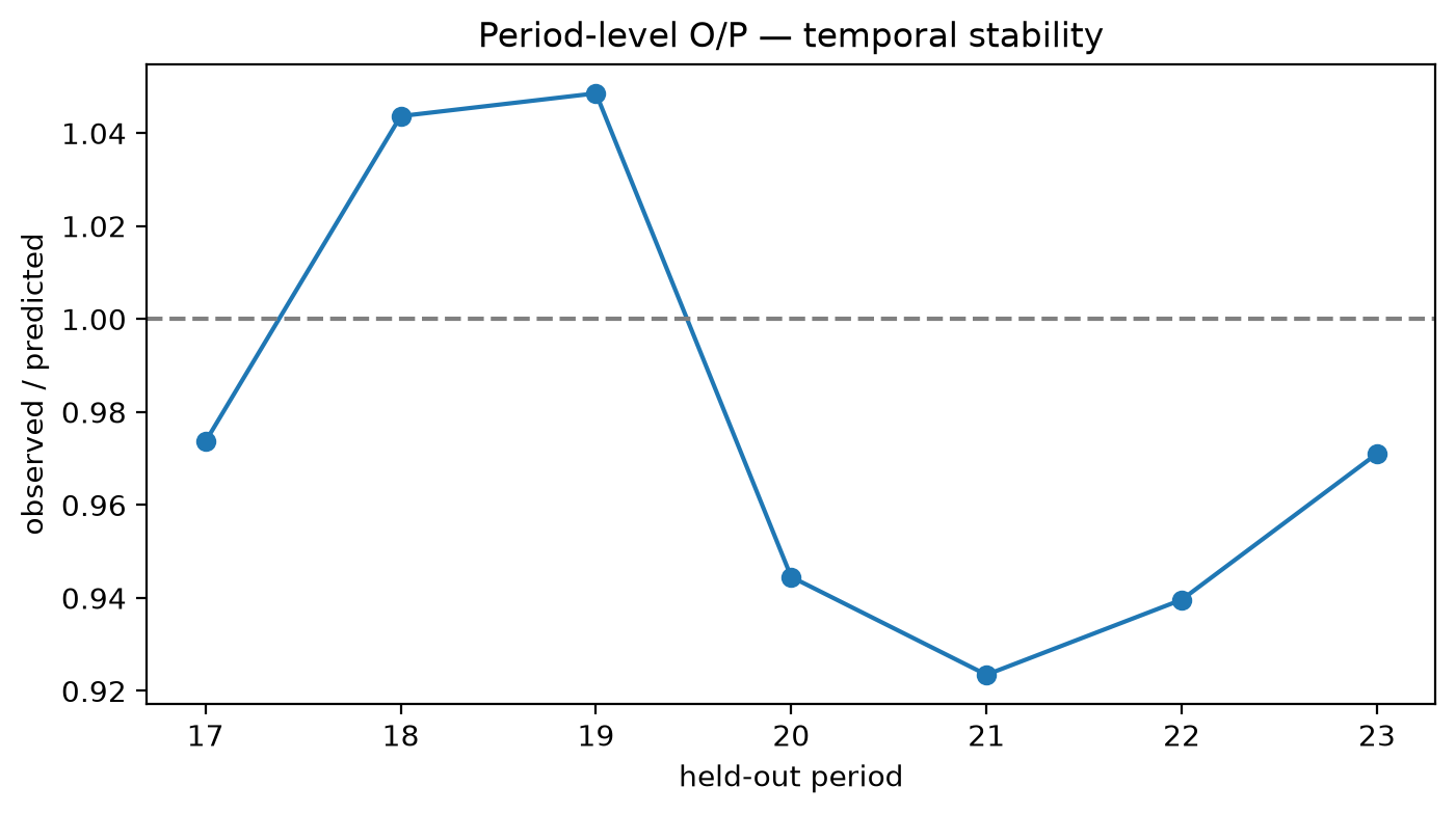
freMTPL2 has no genuine policy-time field, so this chapter builds a small synthetic portfolio with a real period column and exercises the pieces that only make sense on ordered data: a temporal experiment split and the period-level stability_table.

This is an optional, network-free recipe. The data-generating relationships are stationary: no inflation, drift, or structural break is introduced. One model is fitted once and evaluated by later period. The chapter demonstrates chronological partitioning and period summaries, not stability under refitting or robustness to changes in the insured population.

The split trains on earlier periods and tests on later ones. If the requested boundary falls inside a period, every row with that equal timestamp stays on the same side, and missing periods are rejected. The stability table then reports exposure, observed and predicted totals, O/P, Gini, deviance, and \(D^2\) per period on the held-out rows.

rng = np.random.default_rng(RANDOM_STATE)
n_policies = 20_000

exposure = rng.uniform(0.5, 1.0, n_policies)
driver_age = rng.integers(18, 90, n_policies)
vehicle_age = rng.integers(0, 25, n_policies)
region = rng.choice(["urban", "suburban", "rural"], n_policies, p=[0.4, 0.4, 0.2])
period = np.repeat(np.arange(24), np.ceil(n_policies / 24).astype(int))[:n_policies]

frequency = (
    0.10
    * np.where(driver_age < 25, 1.6, np.where(driver_age > 65, 1.3, 1.0))
    * np.where(region == "urban", 1.4, np.where(region == "rural", 0.6, 1.0))
    * (1.0 + 0.03 * vehicle_age)
)
claim_count = rng.poisson(frequency * exposure)
mean_severity = 2_500 * (1.0 + 0.02 * vehicle_age)
claim_amount = np.zeros(n_policies)
has_claim = claim_count > 0
claim_amount[has_claim] = (
    rng.gamma(3.0, mean_severity[has_claim] / 3.0) * claim_count[has_claim]
)

portfolio = pd.DataFrame(
    {
        "period": period,
        "driver_age": driver_age,
        "vehicle_age": vehicle_age,
        "region": region,
        "exposure": exposure,
        "claim_count": claim_count,
        "claim_amount": claim_amount,
    }
)
portfolio_path = ARTIFACT_DIR / "temporal_portfolio.parquet"
portfolio.to_parquet(portfolio_path, index=False)
pd.DataFrame(
    {
        "policies": [len(portfolio)],
        "periods": [portfolio["period"].nunique()],
        "observed_pure_premium": [
            portfolio["claim_amount"].sum() / portfolio["exposure"].sum()
        ],
    }
)

	policies	periods	observed_pure_premium
0	20000	24	536.871643

The run records row positions, so use .iloc even when the portfolio is indexed by policy IDs.

config = ExperimentConfig(
    name="temporal-demo",
    data_path=str(portfolio_path),
    spec=DatasetSpec(
        target="claim_amount",
        exposure="exposure",
        claim_count="claim_count",
        time_col="period",
    ),
    features=["driver_age", "vehicle_age", "region"],
    split="temporal",
    test_size=0.25,
    random_state=RANDOM_STATE,
    models={
        "tweedie-glm": ModelSpec(
            kind="glm",
            params={
                "family": "tweedie",
                "link": "log",
                "tweedie_power": 1.5,
                "alpha": 0.001,
            },
        ),
    },
)
run, estimators = run_experiment(config, return_estimators=True)

train_periods = portfolio.iloc[list(run.train_indices)]["period"].unique()
test_periods = portfolio.iloc[list(run.test_indices)]["period"].unique()
assert train_periods.max() < test_periods.min()
assert len(train_periods) + len(test_periods) == 24
print(f"train periods: {train_periods.min()}–{train_periods.max()}; "
      f"test periods: {test_periods.min()}–{test_periods.max()}")

train periods: 0–16; test periods: 17–23

test_frame = portfolio.iloc[list(run.test_indices)].copy()
y_test = test_frame["claim_amount"].to_numpy()
w_test = test_frame["exposure"].to_numpy()
prediction = np.asarray(
    estimators["tweedie-glm"].predict(test_frame[[*config.features, "exposure"]])
)

stability = stability_table(
    y_test,
    prediction,
    w_test,
    periods=test_frame["period"].to_numpy(),
)
assert len(stability) == len(test_periods)
np.testing.assert_allclose(stability["exposure"].sum(), w_test.sum())
np.testing.assert_allclose(stability["claim_amount"].sum(), y_test.sum())
np.testing.assert_allclose(stability["predicted_claim_amount"].sum(), prediction @ w_test)
display(stability[["period", "exposure", "claim_amount", "predicted_claim_amount"]]
        .rename(columns={"claim_amount": "Observed claims", "predicted_claim_amount": "Predicted claims"}))
display(stability[["period", "o_p_ratio", "gini", "deviance", "d2"]]
        .rename(columns={"o_p_ratio": "O/P", "gini": "Gini", "deviance": "Deviance", "d2": "D²"}))

	period	exposure	Observed claims	Predicted claims
0	17	629.610143	328240.019243	337127.810728
1	18	625.956247	353809.846410	339006.841020
2	19	627.340462	357366.930879	340815.923249
3	20	627.409667	319615.347469	338384.677681
4	21	628.986166	310861.802482	336619.234144
5	22	624.378916	316079.301979	336387.635717
6	23	618.158719	334661.722444	344642.101786

	period	O/P	Gini	Deviance	D²
0	17	0.973637	0.284433	113.321079	0.044788
1	18	1.043666	0.239534	124.805032	0.030456
2	19	1.048563	0.305434	122.568949	0.049626
3	20	0.944533	0.189188	116.864525	0.020964
4	21	0.923482	0.161631	118.180268	0.014086
5	22	0.939628	0.187239	118.636773	0.023453
6	23	0.971041	0.223218	115.287789	0.031381

with plt.style.context("default"):
    fig, ax = plt.subplots(figsize=(8, 4))
    ax.plot(stability["period"], stability["o_p_ratio"], marker="o", label="O/P")
    ax.axhline(1.0, color="grey", linestyle="--")
    ax.set_xlabel("held-out period")
    ax.set_ylabel("observed / predicted")
    ax.set_title("Period-level O/P — temporal stability")
    fig.savefig(ARTIFACT_DIR / "temporal_op.png", bbox_inches="tight")
    plt.show()

Period O/P drifts are read together with exposure and claim totals per row: a single volatile period with little exposure deserves less weight than a stable drift across heavy periods. Use temporal_split-backed configs whenever the portfolio carries any sortable period; without one, report non-temporal held-out diagnostics instead.