5  Scoring and tariff export

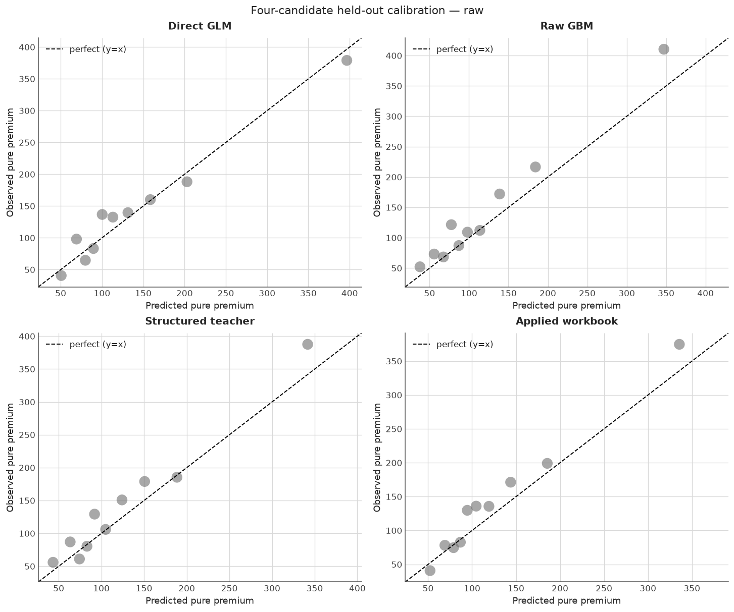
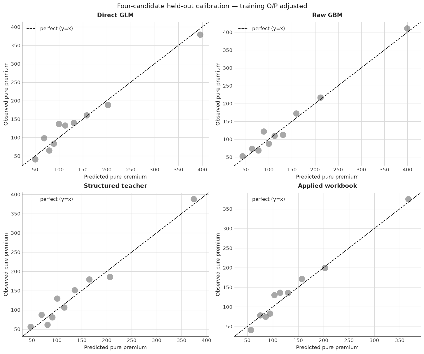
The scoring interface remains estimator.predict(raw_frame). No scoring service or persistence layer is required. The frame below contains only rating features and exposure. Keep the policy ID alongside the results so each price can be traced back to its inputs; it is not a predictor. We retain raw rates and training O/P adjusted rates, following the prediction-scale convention.

portfolio = load_portfolio()
glm_config, gbm_config = make_experiment_configs(str(PORTFOLIO_PATH))
glm_run, glm_estimators = run_experiment(glm_config, return_estimators=True)
gbm_run, gbm_estimators = run_experiment(gbm_config, return_estimators=True)
estimators = {**glm_estimators, **gbm_estimators}
train_frame = portfolio.iloc[list(glm_run.train_indices)].copy()
test_frame = portfolio.iloc[list(glm_run.test_indices)].copy()
y_train = train_frame["claim_amount"].to_numpy()
w_train = train_frame["exposure"].to_numpy()
y_test = test_frame["claim_amount"].to_numpy()
w_test = test_frame["exposure"].to_numpy()
raw_predict_columns = [*FEATURES, "exposure"]
special_predict_columns = [*FEATURES, "exposure", "claim_amount", "claim_count"]

recalibration_factors = {}
for name, estimator in estimators.items():
    pred_train = np.asarray(estimator.predict(train_frame[raw_predict_columns]), dtype=float)
    assert np.isfinite(pred_train).all() and (pred_train > 0).all()
    factor = op_ratio(y_train, pred_train, w_train)
    assert np.isfinite(factor) and factor > 0
    recalibration_factors[name] = factor

scoring_frame = portfolio[raw_predict_columns].copy()
scored = portfolio[["policy_id", "exposure"]].copy()

for model_name, estimator in estimators.items():
    raw_rate = np.asarray(estimator.predict(scoring_frame), dtype=float)
    adjusted_rate = raw_rate * recalibration_factors[model_name]
    assert len(raw_rate) == len(scoring_frame)
    assert np.isfinite(raw_rate).all() and (raw_rate > 0).all()
    for scale, rate in [("raw", raw_rate), ("adjusted", adjusted_rate)]:
        scored[f"{model_name}__{scale}_rate"] = rate
        scored[f"{model_name}__{scale}_expected_period_cost"] = rate * scored["exposure"]

print("Training O/P adjusted rates (EUR per policy-year)")
display(scored.filter(like="__adjusted_rate").describe().T[["mean", "min", "50%", "max"]])

Training O/P adjusted rates (EUR per policy-year)

	mean	min	50%	max
direct-tweedie-glm__adjusted_rate	153.626700	12.345824	113.951167	2794.964164
tweedie-lightgbm__adjusted_rate	152.143669	11.337178	113.857845	4863.010143

5.1 Export the direct GLM

You now have a rate for each policy without supplying its outcomes. Multiply a rate by that policy’s exposure to get expected claim cost for its insured period. Columns ending in __raw_rate and __adjusted_rate are EUR per policy-year; __raw_expected_period_cost and __adjusted_expected_period_cost are EUR for that policy’s insured period. “Adjusted” always means the frozen training O/P multiplier, not a commercial premium loading. The scoring frame reuses known policies to demonstrate the interface; this is not a second performance evaluation.

If a multiplicative workbook is the deliverable, the direct GLM already provides one. This export uses its raw rates, so the training multiplier in scored is not embedded in the workbook:

direct_tariff_path = ARTIFACT_DIR / "direct_tweedie_tariff.xlsx"
export_tariff(
    glm_estimators["direct-tweedie-glm"], direct_tariff_path,
    X=train_frame[special_predict_columns], recalibrate=False,
)
direct_sheets = pd.read_excel(direct_tariff_path, sheet_name=None)
assert not direct_sheets["base_rate"].iloc[0]["recalibrated"]
print("Direct GLM workbook — raw rates (EUR per policy-year)")
display(direct_sheets["base_rate"][["base_rate", "recalibrated"]].T)
display(direct_sheets["factors"].head(10))

Direct GLM workbook — raw rates (EUR per policy-year)

	0
base_rate	48.05387
recalibrated	False

	feature	level	multiplicative_factor	application
0	driver_age	(-inf, 21.5)	1.000000	multiply_by_factor_matching_level
1	driver_age	[21.5, 24.5)	0.446789	multiply_by_factor_matching_level
2	driver_age	[24.5, 27.5)	0.387670	multiply_by_factor_matching_level
3	driver_age	[27.5, 54.5)	0.489958	multiply_by_factor_matching_level
4	driver_age	[54.5, 71.5)	0.473482	multiply_by_factor_matching_level
5	driver_age	[71.5, inf)	0.749925	multiply_by_factor_matching_level
6	driver_age	Missing	0.557837	multiply_by_factor_matching_level
7	vehicle_age	(-inf, 2.5)	1.000000	multiply_by_factor_matching_level
8	vehicle_age	[2.5, 5.5)	0.909299	multiply_by_factor_matching_level
9	vehicle_age	[5.5, 6.5)	0.977541	multiply_by_factor_matching_level

5.2 Work through one policy price

Select the held-out policy with the lowest policy ID. This fixed rule uses neither claims nor predicted cost. Display its original rating inputs beside the levels assigned by the direct GLM’s fitted training bins and groups. Exposure is the insured fraction of a year; it converts a rate into period cost and does not receive a tariff factor.

The workbook application below reuses the same factor-reading recipe as the optional distillation example. It still needs the fitted preprocessing pipeline: this is not standalone reconstruction from the Excel mappings sheet. Retain that fitted pipeline with the workbook.

def tariff_from_sheets(workbook_sheets):
    numeric_factors = {}
    categorical_factors = {}
    for row in workbook_sheets["factors"].itertuples(index=False):
        if row.level == "_per_unit":
            numeric_factors[row.feature] = float(np.log(row.multiplicative_factor))
        else:
            categorical_factors.setdefault(row.feature, {})[str(row.level)] = float(
                row.multiplicative_factor
            )
    return {
        "base_rate": float(workbook_sheets["base_rate"].iloc[0]["base_rate"]),
        "numeric": numeric_factors,
        "categorical": categorical_factors,
    }

worked_policy = test_frame[["policy_id", *raw_predict_columns]].nsmallest(1, "policy_id")
worked_inputs = worked_policy[raw_predict_columns]
direct_pipeline = glm_estimators["direct-tweedie-glm"]
worked_levels = direct_pipeline[:-1].transform(worked_inputs)
direct_tariff = tariff_from_sheets(direct_sheets)

# All nine predictors in this configuration become categorical bins/groups.
assert not direct_tariff["numeric"]
worked_factors = pd.DataFrame({
    "Rating input": FEATURES,
    "Raw value": [worked_inputs.iloc[0][feature] for feature in FEATURES],
    "Fitted level": [str(worked_levels.iloc[0][feature]) for feature in FEATURES],
    "Selected factor": [
        direct_tariff["categorical"][feature][str(worked_levels.iloc[0][feature])]
        for feature in FEATURES
    ],
})
display(worked_policy[["policy_id", "exposure"]].T)
display(worked_factors)

	7
policy_id	811.00
exposure	0.76

	Rating input	Raw value	Fitted level	Selected factor
0	driver_age	44	[27.5, 54.5)	0.489958
1	vehicle_age	0	(-inf, 2.5)	1.000000
2	bonus_malus	50	(-inf, 51.5)	1.000000
3	density	3317	[2676.5, inf)	2.509551
4	region	R93	group_6	1.989918
5	vehicle_brand	B12	group_1	1.066475
6	veh_power	5	group_1	1.036693
7	veh_gas	'Regular'	'Regular'	1.000000
8	area	E	E	0.938247

Multiply the workbook base by every selected factor, including reference levels whose factor is one:

\[ \begin{aligned} \text{raw rate} &= \text{workbook base} \times \prod_j \text{selected factor}_j, \\ \text{adjusted rate} &= \text{raw rate} \times \text{training O/P}. \end{aligned} \]

worked_price = worked_policy[["policy_id", "exposure"]].copy()
worked_price["workbook_base_rate"] = direct_tariff["base_rate"]
worked_price["selected_factor_product"] = worked_factors["Selected factor"].prod()
worked_price["raw_rate"] = (
    worked_price["workbook_base_rate"] * worked_price["selected_factor_product"]
)
worked_price["frozen_training_op"] = recalibration_factors["direct-tweedie-glm"]
worked_price["adjusted_rate"] = (
    worked_price["raw_rate"] * worked_price["frozen_training_op"]
)
for scale in ["raw", "adjusted"]:
    worked_price[f"{scale}_expected_period_cost"] = (
        worked_price[f"{scale}_rate"] * worked_price["exposure"]
    )

display(
    worked_price.T.rename(columns={worked_price.index[0]: "Worked policy"})
)

	Worked policy
policy_id	811.000000
exposure	0.760000
workbook_base_rate	48.053870
selected_factor_product	2.538096
raw_rate	121.965359
frozen_training_op	0.998170
adjusted_rate	121.742112
raw_expected_period_cost	92.693673
adjusted_expected_period_cost	92.524005

Read the last two rows as expected claim costs in EUR for this exposure, before and after the training adjustment. The base and both rates are EUR per policy-year; the factor product and training O/P are unitless. The workbook remains on the raw scale: the training multiplier is applied externally, exactly as in scored. It balances training totals, without guaranteeing this policy’s cost or held-out calibration. These are expected claims on the tutorial’s capped loss layer, before expenses, profit, taxes, or other commercial loadings.

For a tariff review, check the base rate, factor levels, mappings, loss layer, and raw prediction scale against the GLM diagnostics. The full-portfolio and segment limitations remain. You can stop here with a scored portfolio and a direct GLM workbook for review. Use reporting to record the run, or continue below if a GBM must be represented as a tariff.

5.3 Optional extension: distillation and workbook evaluation

The remaining sections evaluate a GBM-derived workbook, including its agreement with its student model and its performance against held-out claims.

5.4 Distil the GBM into an executable tariff

A tree model is not itself a multiplicative tariff. distill_gbm fits a log-link GLM student to a GBM teacher’s predictions on the experiment’s training rows, then measures fidelity on the untouched test rows. It copies the already-fitted preprocessing, so bins and group mappings are not relearned from the holdout. The teacher here is the raw, unscaled tariff-structured Tweedie LightGBM (tweedie-lightgbm-tariff), before the chart adjustment: the student lives in the same binned/grouped feature space. Fidelity measures agreement with this teacher; it does not establish performance against claims.

Construct this extra candidate here: copy the raw GBM’s fixed tree settings into a separate experiment with the GLM’s preprocessing and split. This is a new fit, with the same training rows and learned rating structure as the GLM; it does not change either main-path model.

teacher_config = glm_config.model_copy(update={
    "name": "fremtpl2-structured-teacher",
    "models": {"tweedie-lightgbm-tariff": gbm_config.models["tweedie-lightgbm"].model_copy(deep=True)},
})
teacher_run, teacher_estimators = run_experiment(teacher_config, return_estimators=True)
teacher_pipeline = teacher_estimators["tweedie-lightgbm-tariff"]

assert teacher_run.data_fingerprint == glm_run.data_fingerprint
assert teacher_run.train_indices == glm_run.train_indices
assert teacher_run.test_indices == glm_run.test_indices
teacher_train_rate = teacher_pipeline.predict(train_frame[raw_predict_columns])
teacher_factor = op_ratio(y_train, teacher_train_rate, w_train)
assert np.isfinite(teacher_factor) and teacher_factor > 0
np.testing.assert_allclose(op_ratio(y_train, teacher_factor * teacher_train_rate, w_train), 1)

The workbook contains the same base_rate, factors, and mappings sheets as a direct GLM export. Here recalibrate=False is deliberate: applying the workbook reproduces the student exactly. The student approximates the GBM teacher; the workbook does not reproduce the teacher exactly. Export receives only the training frame for feature metadata. The held-out fidelity metadata still measures agreement with the teacher, not with claims.

tariff_path = ARTIFACT_DIR / "distilled_tweedie_tariff.xlsx"
tariff_X = portfolio[
    [*FEATURES, "exposure", "claim_amount", "claim_count"]
]
fit_X = train_frame[special_predict_columns]
validation_X = test_frame[special_predict_columns]
distilled_pipeline = distill_gbm(teacher_pipeline, fit_X, validation_X)

export_tariff(
    distilled_pipeline,
    tariff_path,
    X=fit_X,
    recalibrate=False,
)

sheets = pd.read_excel(tariff_path, sheet_name=None)

pd.testing.assert_frame_equal(fit_X, tariff_X.iloc[list(glm_run.train_indices)])
pd.testing.assert_frame_equal(validation_X, tariff_X.iloc[list(glm_run.test_indices)])
assert list(sheets) == ["base_rate", "factors", "mappings"]
assert sheets["base_rate"].iloc[0]["distilled_from"] == "RiskGBM"
assert not sheets["base_rate"].iloc[0]["recalibrated"]
print("Distilled workbook — raw student rates (EUR per policy-year)")
display(sheets["base_rate"].T)
display(sheets["factors"].head(20))
display(sheets["mappings"].head(20))

Distilled workbook — raw student rates (EUR per policy-year)

	0
base_rate	51.015377
family	tweedie
link	log
intercept_	5.225353
recalibrated	False
distilled_from	RiskGBM
teacher_objective	tweedie
teacher_student_deviance	0.661562
student_teacher_total_ratio	1.003165

	feature	level	multiplicative_factor	application
0	driver_age	(-inf, 21.5)	1.000000	multiply_by_factor_matching_level
1	driver_age	[21.5, 24.5)	0.561933	multiply_by_factor_matching_level
2	driver_age	[24.5, 27.5)	0.493566	multiply_by_factor_matching_level
3	driver_age	[27.5, 54.5)	0.618848	multiply_by_factor_matching_level
4	driver_age	[54.5, 71.5)	0.624068	multiply_by_factor_matching_level
5	driver_age	[71.5, inf)	0.761103	multiply_by_factor_matching_level
6	driver_age	Missing	0.658489	multiply_by_factor_matching_level
7	vehicle_age	(-inf, 2.5)	1.000000	multiply_by_factor_matching_level
8	vehicle_age	[2.5, 5.5)	0.980187	multiply_by_factor_matching_level
9	vehicle_age	[5.5, 6.5)	0.974645	multiply_by_factor_matching_level
10	vehicle_age	[6.5, 7.5)	0.999024	multiply_by_factor_matching_level
11	vehicle_age	[7.5, 12.5)	0.939047	multiply_by_factor_matching_level
12	vehicle_age	[12.5, 15.5)	0.736423	multiply_by_factor_matching_level
13	vehicle_age	[15.5, 18.5)	0.708853	multiply_by_factor_matching_level
14	vehicle_age	[18.5, inf)	0.464310	multiply_by_factor_matching_level
15	vehicle_age	Missing	0.826254	multiply_by_factor_matching_level
16	bonus_malus	(-inf, 51.5)	1.000000	multiply_by_factor_matching_level
17	bonus_malus	[51.5, 57.5)	1.403540	multiply_by_factor_matching_level
18	bonus_malus	[57.5, 63.5)	2.322182	multiply_by_factor_matching_level
19	bonus_malus	[63.5, 90.5)	2.034211	multiply_by_factor_matching_level

	feature	role	dtype	levels	n_levels	reference_level	mapping
0	driver_age	categorical	category	(-inf, 21.5), [21.5, 24.5), [24.5, 27.5), [27....	7	(-inf, 21.5)	NaN
1	vehicle_age	categorical	category	(-inf, 2.5), [2.5, 5.5), [5.5, 6.5), [6.5, 7.5...	9	(-inf, 2.5)	NaN
2	bonus_malus	categorical	category	(-inf, 51.5), [51.5, 57.5), [57.5, 63.5), [63....	7	(-inf, 51.5)	NaN
3	density	categorical	category	(-inf, 18.5), [18.5, 375.5), [375.5, 2351.0), ...	6	(-inf, 18.5)	NaN
4	region	categorical	category	group_0, group_1, group_2, group_3, group_4, g...	9	group_0	NaN
5	vehicle_brand	categorical	category	group_0, group_1, B1, B4, B5, B13, group_6, B1...	9	group_0	NaN
6	veh_power	categorical	category	group_0, group_1, 7, group_3, 11, 10, 12, grou...	9	group_0	NaN
7	veh_gas	categorical	category	'Regular', 'Diesel', Other	3	'Regular'	NaN
8	area	categorical	category	B, A, C, D, F, E, Other	7	B	NaN
9	driver_age	binned	category	(-inf, 21.5), [21.5, 24.5), [24.5, 27.5), [27....	7	NaN	21.5, 24.5, 27.5, 54.5, 71.5
10	vehicle_age	binned	category	(-inf, 2.5), [2.5, 5.5), [5.5, 6.5), [6.5, 7.5...	9	NaN	2.5, 5.5, 6.5, 7.5, 12.5, 15.5, 18.5
11	bonus_malus	binned	category	(-inf, 51.5), [51.5, 57.5), [57.5, 63.5), [63....	7	NaN	51.5, 57.5, 63.5, 90.5, 95.5
12	density	binned	category	(-inf, 18.5), [18.5, 375.5), [375.5, 2351.0), ...	6	NaN	18.5, 375.5, 2351.0, 2676.5
13	region	grouped	category	group_0, group_1, group_2, group_3, group_4, g...	9	NaN	'R11' -> 'group_4'; 'R21' -> 'group_7'; 'R22' ...
14	vehicle_brand	grouped	category	group_0, group_1, B1, B4, B5, B13, group_6, B1...	9	NaN	'B1' -> 'B1'; 'B10' -> 'group_6'; 'B11' -> 'B1...
15	veh_power	grouped	category	group_0, group_1, 7, group_3, 11, 10, 12, grou...	9	NaN	'10' -> '10'; '11' -> '11'; '12' -> '12'; '13'...
16	veh_gas	grouped	category	'Regular', 'Diesel', Other	3	NaN	"'Diesel'" -> "'Diesel'"; "'Regular'" -> "'Reg...
17	area	grouped	category	B, A, C, D, F, E, Other	7	NaN	'A' -> 'A'; 'B' -> 'B'; 'C' -> 'C'; 'D' -> 'D'...

The following application still uses the student’s fitted preprocessing pipeline. It verifies workbook factors after transformation; it does not reconstruct standalone scoring from the Excel mappings sheet. Retain that pipeline with the workbook for this recipe.

workbook_tariff = tariff_from_sheets(sheets)
transformed_validation = distilled_pipeline[:-1].transform(validation_X)
teacher_rate = np.asarray(teacher_pipeline.predict(validation_X), dtype=float)
raw_test_predictions = {
    name: np.asarray(estimator.predict(test_frame[raw_predict_columns]), dtype=float)
    for name, estimator in estimators.items()
}
np.testing.assert_allclose(teacher_rate, teacher_pipeline.predict(test_frame[raw_predict_columns]))
student_rate = np.asarray(distilled_pipeline.predict(validation_X), dtype=float)
workbook_rate = apply_tariff(workbook_tariff, transformed_validation)

for frame in [fit_X, validation_X]:
    applied = apply_tariff(workbook_tariff, distilled_pipeline[:-1].transform(frame))
    student = np.asarray(distilled_pipeline.predict(frame), dtype=float)
    assert np.isfinite(applied).all() and (applied > 0).all()
    np.testing.assert_allclose(applied, student, rtol=1e-6, atol=1e-8)
for step in ["binner", "grouper"]:
    original = teacher_pipeline.named_steps[step].mapping_
    copied = distilled_pipeline.named_steps[step].mapping_
    assert original.keys() == copied.keys()
    for name in original:
        if step == "binner":
            np.testing.assert_array_equal(original[name], copied[name])
        else:
            assert original[name] == copied[name]

5.5 Teacher–student fidelity, separately from claims performance

Here the target is the teacher’s predicted rate, not observed claims. Weighted Tweedie deviance at power 1.5 is zero for exact reproduction; the student/teacher predicted-total ratio is one for equal totals. Neither establishes accuracy against losses or segment calibration.

fidelity = {
    "teacher_student_deviance": mean_tweedie_deviance(
        teacher_rate, student_rate, sample_weight=w_test, power=1.5,
    ),
    "student_teacher_total_ratio": (student_rate @ w_test) / (teacher_rate @ w_test),
}
for key, value in fidelity.items():
    np.testing.assert_allclose(value, distilled_pipeline.distillation_metrics_[key])
    np.testing.assert_allclose(value, sheets["base_rate"].iloc[0][key])
display(pd.DataFrame([fidelity]).assign(target="raw teacher rates", partition="test"))

	teacher_student_deviance	student_teacher_total_ratio	target	partition
0	0.661562	1.003165	raw teacher rates	test

5.6 Four candidates against the same held-out claims

The applied workbook is the fourth candidate. Its rates come from the workbook factors applied after the student’s fitted preprocessing, not from a teacher prediction. All four rows use exactly the same test claims and exposure. Deviance is exposure-weighted Tweedie at power 1.5; \(D^2\) uses the same constant held-out mean reference as above. Concentration Gini measures ranking only.

The second table applies each candidate’s own frozen training O/P. For the workbook, compute that factor from applied workbook predictions on training rows; it is an external multiplier, not a change to the exported base or factors. It balances training totals and can improve or worsen held-out diagnostics.

workbook_train_rate = apply_tariff(workbook_tariff, distilled_pipeline[:-1].transform(fit_X))
workbook_factor = op_ratio(y_train, workbook_train_rate, w_train)
assert np.isfinite(workbook_factor) and workbook_factor > 0
np.testing.assert_allclose(op_ratio(y_train, workbook_factor * workbook_train_rate, w_train), 1)
final_factors = {
    "Direct GLM": recalibration_factors["direct-tweedie-glm"],
    "Raw GBM": recalibration_factors["tweedie-lightgbm"],
    "Structured teacher": teacher_factor,
    "Applied workbook": workbook_factor,
}
final_raw_predictions = {
    "Direct GLM": raw_test_predictions["direct-tweedie-glm"],
    "Raw GBM": raw_test_predictions["tweedie-lightgbm"],
    "Structured teacher": teacher_rate,
    "Applied workbook": workbook_rate,
}
final_adjusted_predictions = {
    name: prediction * final_factors[name] for name, prediction in final_raw_predictions.items()
}
final_rows = []
for scale, predictions in [("raw", final_raw_predictions),
                           ("training O/P adjusted", final_adjusted_predictions)]:
    for name, prediction in predictions.items():
        assert prediction.shape == y_test.shape
        assert np.isfinite(prediction).all() and (prediction > 0).all()
        values = holdout_diagnostics(y_test, w_test, prediction)
        np.testing.assert_allclose(values["gini_test"], gini(y_test, final_raw_predictions[name], w_test))
        np.testing.assert_allclose(
            values["op_ratio_test"], y_test.sum() / (prediction @ w_test),
        )
        final_rows.append({
            "model": name, "prediction_scale": scale, **values,
            "predicted_claim_amount": prediction @ w_test,
            "observed_claim_amount": y_test.sum(), "exposure": w_test.sum(),
            "frozen_training_factor": final_factors[name],
        })
final_metrics = pd.DataFrame(final_rows)
for scale in ["raw", "training O/P adjusted"]:
    table = final_metrics[final_metrics.prediction_scale == scale]
    assert len(table) == 4
    assert table.observed_claim_amount.nunique() == table.exposure.nunique() == 1
    print(scale)
    display(table.set_index("model")[["gini_test", "op_ratio_test", "deviance_test", "d2_test"]]
            .rename(columns={"gini_test": "Gini", "op_ratio_test": "O/P",
                             "deviance_test": "Deviance", "d2_test": "D²"}))
    display(table.set_index("model")[["predicted_claim_amount", "frozen_training_factor"]]
            .rename(columns={"predicted_claim_amount": "Predicted claims",
                             "frozen_training_factor": "Training factor"}))
print(f"Shared test claims: {y_test.sum():,.2f}; exposure: {w_test.sum():,.2f}")
final_metrics.to_csv(ARTIFACT_DIR / "tariff_claims_comparison.csv", index=False)

raw

	Gini	O/P	Deviance	D²
model
Direct GLM	0.309850	1.022067	75.338331	0.048954
Raw GBM	0.341982	1.178104	74.721321	0.056743
Structured teacher	0.319185	1.123572	75.285399	0.049622
Applied workbook	0.319752	1.120027	75.279827	0.049693

	Predicted claims	Training factor
model
Direct GLM	9.817210e+06	0.998170
Raw GBM	8.516946e+06	1.150219
Structured teacher	8.930316e+06	1.096248
Applied workbook	8.958580e+06	1.093725

training O/P adjusted

	Gini	O/P	Deviance	D²
model
Direct GLM	0.309850	1.023942	75.340078	0.048932
Raw GBM	0.341982	1.024243	74.405403	0.060731
Structured teacher	0.319185	1.024925	75.119374	0.051718
Applied workbook	0.319752	1.024048	75.146789	0.051372

	Predicted claims	Training factor
model
Direct GLM	9.799241e+06	0.998170
Raw GBM	9.796356e+06	1.150219
Structured teacher	9.789838e+06	1.096248
Applied workbook	9.798220e+06	1.093725

Shared test claims: 10,033,849.49; exposure: 70,511.87

5.7 Calibration and ranking of the applied tariff

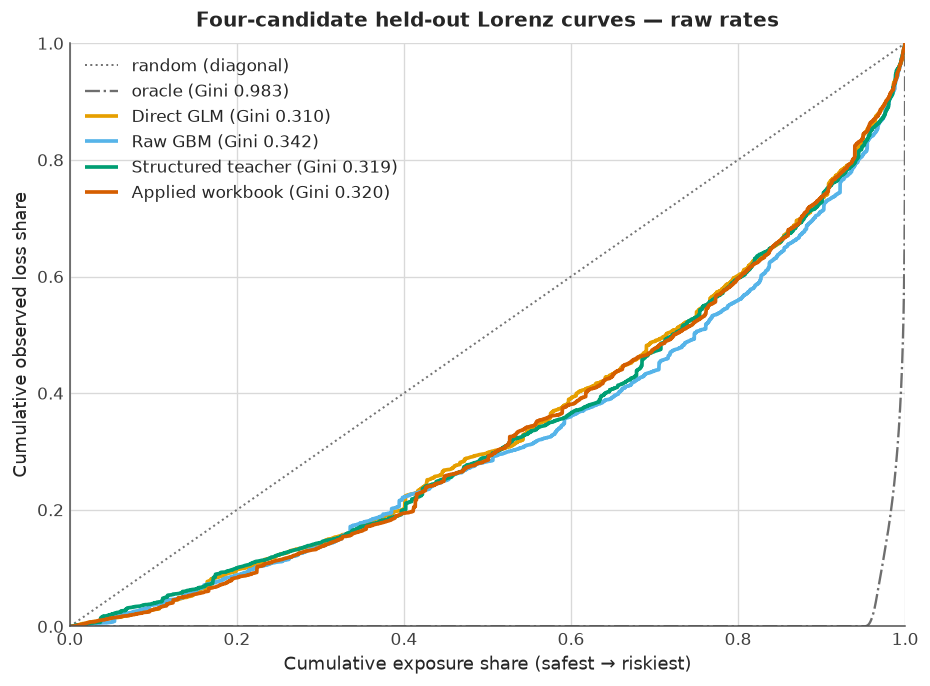
Each calibration panel compares observed and predicted rates in that candidate’s exposure-weighted prediction deciles. The diagonal means agreement in level. The Lorenz overlay uses raw rates; positive training multipliers preserve every curve, as checked above. Crossing curves do not establish ranking dominance.

final_colors = model_colors(list(final_raw_predictions))
with azoic_style():
    for scale, predictions in [("raw", final_raw_predictions),
                               ("training O/P adjusted", final_adjusted_predictions)]:
        fig, axes = plt.subplots(2, 2, figsize=(12, 10), layout="constrained")
        for (name, prediction), ax in zip(predictions.items(), axes.flat, strict=True):
            table = calibration_table(y_test, prediction, w_test, n_bins=10)
            np.testing.assert_allclose(table.exposure.sum(), w_test.sum())
            np.testing.assert_allclose(table.claim_amount.sum(), y_test.sum())
            np.testing.assert_allclose(table.predicted_claim_amount.sum(), prediction @ w_test)
            plot_calibration(table, ax=ax, title=name)
        fig.suptitle(f"Four-candidate held-out calibration — {scale}")
        suffix = "raw" if scale == "raw" else "adjusted"
        fig.savefig(ARTIFACT_DIR / f"tariff_calibration_{suffix}.png", bbox_inches="tight")
        plt.close(fig)
        display(Image(filename=str(ARTIFACT_DIR / f"tariff_calibration_{suffix}.png"), width=700))
    fig, ax = plt.subplots(figsize=(8, 6))
    plot_lorenz(y_test, final_raw_predictions, w_test, ax=ax, show_oracle=True,
                title="Four-candidate held-out Lorenz curves — raw rates")
    fig.savefig(ARTIFACT_DIR / "tariff_lorenz.png", bbox_inches="tight")
    plt.close(fig)
    display(Image(filename=str(ARTIFACT_DIR / "tariff_lorenz.png"), width=700))

5.8 Compare candidates at each raw age, then inside tariff bins

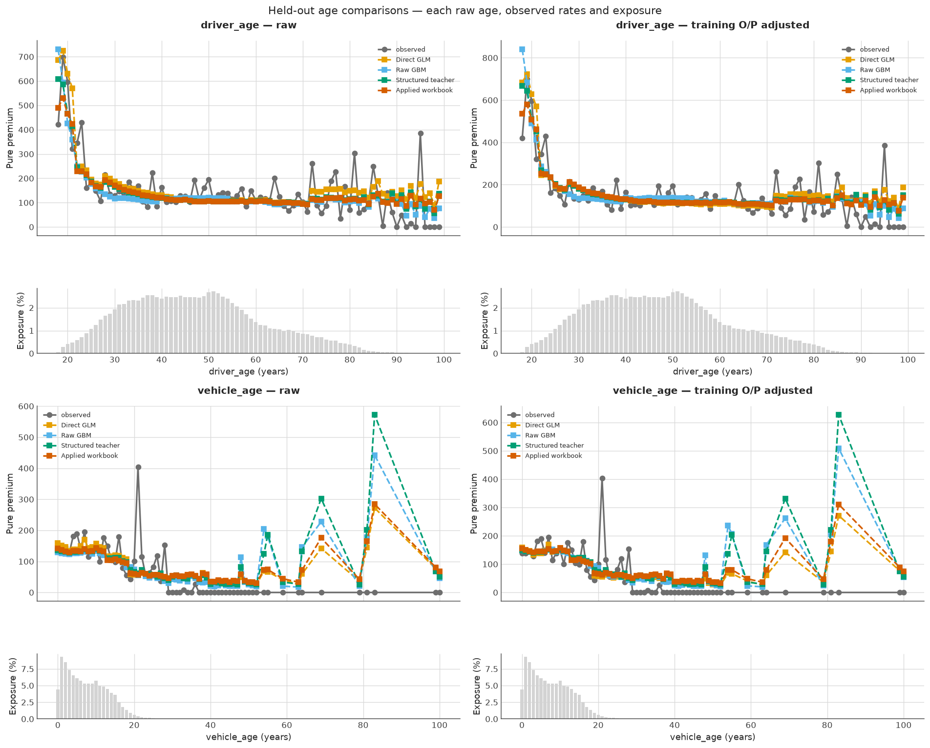
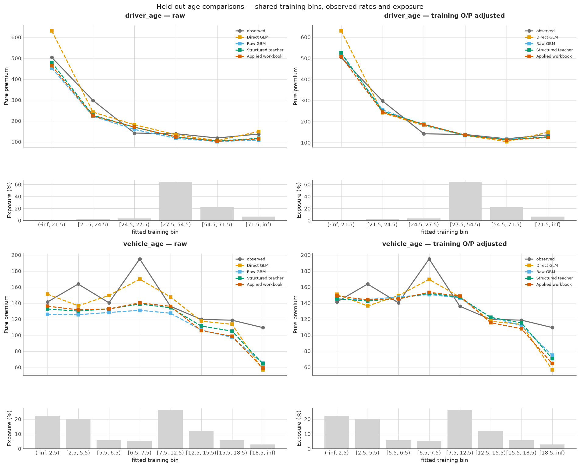
The first figure compares all four candidates at every observed driver and vehicle age. Use it to locate differences that could be hidden by a fitted bin. The second is a supporting tariff view using the direct GLM’s frozen training bins. This also puts the raw-feature GBM in those bins for reporting; it does not alter its inputs or fit new cuts.

Both views reuse the same held-out predictions. Observed rates and exposure are shared across candidates within each view. Raw and training O/P adjusted rates appear in separate columns; “raw” in those column titles means no level adjustment, independently of whether the x-axis uses raw ages or fitted bins. These are portfolio averages, subject to composition and claim variation. Read the sparse tails alongside exposure before interpreting a jagged line.

glm_pipeline = glm_estimators["direct-tweedie-glm"]
fitted_preprocessing = glm_pipeline[:-1]
test_grouped = fitted_preprocessing.transform(test_frame[special_predict_columns])
with azoic_style():
    for grouping, frame, suffix in [
        ("each raw age", test_frame, "raw"),
        ("shared training bins", test_grouped, "grouped"),
    ]:
        fig, axes = plt.subplots(4, 2, figsize=(16, 13), layout="tight",
                                 gridspec_kw={"height_ratios": [3, 1, 3, 1]})
        for row, feature in enumerate(["driver_age", "vehicle_age"]):
            for col, (scale, predictions) in enumerate([
                ("raw", final_raw_predictions),
                ("training O/P adjusted", final_adjusted_predictions),
            ]):
                ax, exposure_ax = axes[2 * row, col], axes[2 * row + 1, col]
                exposure_ax.sharex(ax)
                reference_table = None
                for name, prediction in predictions.items():
                    table = one_way_table(frame, feature, y_test, prediction, w_test, n_bins=None)
                    np.testing.assert_allclose(table.exposure.sum(), w_test.sum())
                    np.testing.assert_allclose(table.claim_amount.sum(), y_test.sum())
                    np.testing.assert_allclose(table.predicted_claim_amount.sum(), prediction @ w_test)
                    if suffix == "raw":
                        np.testing.assert_array_equal(table.level, np.sort(test_frame[feature].unique()))
                    common_columns = ["level", "level_label", "level_center", "exposure",
                                      "claim_amount", "observed_pure_premium"]
                    if reference_table is None:
                        reference_table = table
                        plot_one_way(table, ax=ax, color=final_colors[name], label=name,
                                     exposure="none", title=f"{feature} — {scale}")
                        exposure_ax.bar(ax.lines[0].get_xdata(),
                                        100 * table.exposure / w_test.sum(), color="lightgrey")
                        exposure_ax.set_ylabel("Exposure (%)")
                    else:
                        pd.testing.assert_frame_equal(table[common_columns], reference_table[common_columns])
                        ax.plot(ax.lines[0].get_xdata(), table.predicted_pure_premium,
                                marker="s", linestyle="--", color=final_colors[name], label=name)
                ax.set_title(f"{feature} — {scale}", y=1.02)
                ax.set_xlabel("")
                ax.tick_params(axis="x", labelbottom=False)
                exposure_ax.set_xlabel(f"{feature} (years)" if suffix == "raw" else "fitted training bin")
                ax.legend(fontsize=8)
        fig.suptitle(f"Held-out age comparisons — {grouping}, observed rates and exposure")
        figure_path = ARTIFACT_DIR / f"tariff_age_comparison_{suffix}.png"
        fig.savefig(figure_path, bbox_inches="tight")
        plt.close(fig)
        display(Image(filename=str(figure_path), width=700))

5.9 What is gained and lost in this export?

The workbook gains a multiplicative factor representation. It preserves the student’s rates to the checked numerical tolerance, while approximating the teacher’s predictions. The table below reports workbook minus comparator on claims: negative deviance differences mean lower loss; positive \(D^2\) or Gini differences mean improvement in that statistic. An O/P change must be read against one, not maximized. Predicted-total changes are monetary level changes.

export_differences = []
for scale in ["raw", "training O/P adjusted"]:
    table = final_metrics[final_metrics.prediction_scale == scale].set_index("model")
    for comparator in ["Direct GLM", "Raw GBM", "Structured teacher"]:
        columns = ["deviance_test", "d2_test", "gini_test", "op_ratio_test", "predicted_claim_amount"]
        differences = table.loc["Applied workbook", columns] - table.loc[comparator, columns]
        export_differences.append({"workbook_minus": comparator, "prediction_scale": scale,
                                   **differences.to_dict()})
for scale, table in pd.DataFrame(export_differences).groupby("prediction_scale", sort=False):
    print(scale)
    display(table.drop(columns="prediction_scale").set_index("workbook_minus")
            .rename(columns={"deviance_test": "Deviance", "d2_test": "D²",
                             "gini_test": "Gini", "op_ratio_test": "O/P",
                             "predicted_claim_amount": "Predicted claims"}))

raw

	Deviance	D²	Gini	O/P	Predicted claims
workbook_minus
Direct GLM	-0.058504	0.000739	0.009902	0.097959	-858629.719565
Raw GBM	0.558506	-0.007050	-0.022230	-0.058077	441633.876840
Structured teacher	-0.005572	0.000070	0.000568	-0.003545	28264.838477

training O/P adjusted

	Deviance	D²	Gini	O/P	Predicted claims
workbook_minus
Direct GLM	-0.193290	0.002440	0.009902	0.000107	-1020.832537
Raw GBM	0.741385	-0.009359	-0.022230	-0.000195	1863.595610
Structured teacher	0.027414	-0.000346	0.000568	-0.000877	8382.061566

Distillation may improve or worsen claims performance: approximation error against a teacher is not the same as prediction error against claims. Read the differences alongside calibration and age panels; equal portfolio totals do not imply equal segment rates. This single held-out split gives descriptive evidence, not statistical superiority, stability under refitting, or an automatic choice of production tariff. Adjusted workbook results describe the workbook plus its external training multiplier; the exported workbook itself remains raw.